다익스트라

■ 다익스트라 알고리즘

1) 정의 :

자료구조로 graph 사용,

" 노드 + 가중치를 가진 간선 "을 이용하여 최단경로를 계산

 

2) graph 자료구조 참조

참조 : korshika.tistory.com/42?category=957674

 

3) 시간복잡도 :

O( E * log(E) ) ≒ O( E * log( V) )

> "최대의 경우"

   모든 간선 E에 대해서 dist_history= [ ]가 한번씩 계산이 되기 때문에 

   간선을 queue에 작업하는 평균 시간 복잡도 O( log(E) )를 곱하면

   최대 O( E * log(E) ) 에 비례,

> 일반적으로 노드는 간선보다 적기 때문에,

   O( E * log( V) ) 라고 쓸 수도 있다

 

■  코드 구현

1) 코드 이해코드 설명 참조 : Link

 

2) 코드 - 파이썬

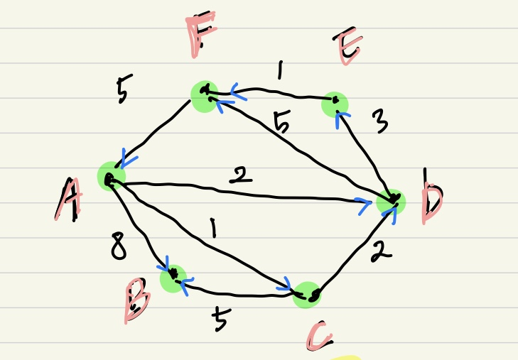
import heapq # 복잡도 N log(N)

/*
# 유향 그래프
graph = {
    'A': {'B': 8, 'C': 1, 'D': 2},
    'B': {},
    'C': {'B': 5, 'D': 2},
    'D': {'E': 3, 'F': 5},
    'E': {'F': 1},
    'F': {'A': 5}
}
*/

def dijkstra(graph, start):
    q = []
    recordDist = {node: float('inf') for node in graph}
    recordDist[start] = 0 # 시작 위치 0 distance
    heapq.heappush(q, [recordDist[start], start])
    
    while q :
        
        curNodeDist, curNodeName = heapq.heappop(q) # 현재에서 가장 비용 낮은 순 탐색
        """
        지금 방문한 node가 queue에 담긴 시점은
        recordDist가 [section-b]에서 업데이트 되기 전일 수 있음
        따라서 [section-a]에서 체크해줌
        """
        
        # [section-a]
        if recordDist[curNodeName] < curNodeDist:
       	    # 여기서 연결된 노드는 더 이상 볼필요가 없음, 이미 갱신되어서
            # 옛날에 queue에 담긴 탐색 결과가 더 비용이 많이 들기 때문
            continue
         
         
         # [section-b]
         for new_dest, new_dist in graph[curNodeName].items():
            total_dist = curNodeDist + new_dist
            if total_dist < recordDist[new_dest]:
                recordDist[new_dest] = total_dist
            	heapq.heappush(q, [total_dist, new_dest])
                
    return recordDist
    

---

3) 예제

> 밑에 예제에서 확인가능 하지만, 유향 그래프로 설정하여도 되고 안해도 됨

> nested dictionary 사용

 

# 유향 그래프
graph = {
    'A': {'B': 8, 'C': 1, 'D': 2},
    'B': {},
    'C': {'B': 5, 'D': 2},
    'D': {'E': 3, 'F': 5},
    'E': {'F': 1},
    'F': {'A': 5}
}

import heapq  # 우선순위 큐 구현을 위함

def dijkstra(graph, start):
  distances = {node: float('inf') for node in graph}  # start로 부터의 거리 값을 저장하기 위함
  distances[start] = 0  # 시작 값은 0이어야 함
  queue = []
  heapq.heappush(queue, [distances[start], start])  # 시작 노드부터 탐색 시작 하기 위함.

  while queue:  # queue에 남아 있는 노드가 없으면 끝
    print(f'graph : {graph}')
    print(f'distances : {distances}')
    print(f'before queue : {queue}')
    current_distance, current_destination = heapq.heappop(queue)  # 탐색 할 노드, 거리를 가져옴.
    print(f'current_distance : {current_distance}, current_destination : {current_destination}')
    print(f'distances[current_destination] : {distances[current_destination]}, current_distance : {current_distance}')

    if distances[current_destination] < current_distance:  # 기존에 있는 거리보다 길다면, 볼 필요도 없음
      continue
    
    for new_destination, new_distance in graph[current_destination].items():
      distance = current_distance + new_distance  # 해당 노드를 거쳐 갈 때 거리
      if distance < distances[new_destination]:  # 알고 있는 거리 보다 작으면 갱신
        print(f'renew {new_destination} from {distances[new_destination]} to {distance}')
        distances[new_destination] = distance
        heapq.heappush(queue, [distance, new_destination])  # 다음 인접 거리를 계산 하기 위해 큐에 삽입
    print(f'next queue : {queue}')
    print('\n'*2)
  return distances
  
print(dijkstra(graph, 'A'))


>>>
graph : {'A': {'B': 8, 'C': 1, 'D': 2}, 'B': {}, 'C': {'B': 5, 'D': 2}, 'D': {'E': 3, 'F': 5}, 'E': {'F': 1}, 'F': {'A': 5}}
distances : {'A': 0, 'B': inf, 'C': inf, 'D': inf, 'E': inf, 'F': inf}
before queue : [[0, 'A']]
current_distance : 0, current_destination : A
distances[current_destination] : 0, current_distance : 0
renew B from inf to 8
renew C from inf to 1
renew D from inf to 2
next queue : [[1, 'C'], [8, 'B'], [2, 'D']]



graph : {'A': {'B': 8, 'C': 1, 'D': 2}, 'B': {}, 'C': {'B': 5, 'D': 2}, 'D': {'E': 3, 'F': 5}, 'E': {'F': 1}, 'F': {'A': 5}}
distances : {'A': 0, 'B': 8, 'C': 1, 'D': 2, 'E': inf, 'F': inf}
before queue : [[1, 'C'], [8, 'B'], [2, 'D']]
current_distance : 1, current_destination : C
distances[current_destination] : 1, current_distance : 1
renew B from 8 to 6
next queue : [[2, 'D'], [8, 'B'], [6, 'B']]



graph : {'A': {'B': 8, 'C': 1, 'D': 2}, 'B': {}, 'C': {'B': 5, 'D': 2}, 'D': {'E': 3, 'F': 5}, 'E': {'F': 1}, 'F': {'A': 5}}
distances : {'A': 0, 'B': 6, 'C': 1, 'D': 2, 'E': inf, 'F': inf}
before queue : [[2, 'D'], [8, 'B'], [6, 'B']]
current_distance : 2, current_destination : D
distances[current_destination] : 2, current_distance : 2
renew E from inf to 5
renew F from inf to 7
next queue : [[5, 'E'], [7, 'F'], [6, 'B'], [8, 'B']]



graph : {'A': {'B': 8, 'C': 1, 'D': 2}, 'B': {}, 'C': {'B': 5, 'D': 2}, 'D': {'E': 3, 'F': 5}, 'E': {'F': 1}, 'F': {'A': 5}}
distances : {'A': 0, 'B': 6, 'C': 1, 'D': 2, 'E': 5, 'F': 7}
before queue : [[5, 'E'], [7, 'F'], [6, 'B'], [8, 'B']]
current_distance : 5, current_destination : E
distances[current_destination] : 5, current_distance : 5
renew F from 7 to 6
next queue : [[6, 'B'], [6, 'F'], [8, 'B'], [7, 'F']]



graph : {'A': {'B': 8, 'C': 1, 'D': 2}, 'B': {}, 'C': {'B': 5, 'D': 2}, 'D': {'E': 3, 'F': 5}, 'E': {'F': 1}, 'F': {'A': 5}}
distances : {'A': 0, 'B': 6, 'C': 1, 'D': 2, 'E': 5, 'F': 6}
before queue : [[6, 'B'], [6, 'F'], [8, 'B'], [7, 'F']]
current_distance : 6, current_destination : B
distances[current_destination] : 6, current_distance : 6
next queue : [[6, 'F'], [7, 'F'], [8, 'B']]



graph : {'A': {'B': 8, 'C': 1, 'D': 2}, 'B': {}, 'C': {'B': 5, 'D': 2}, 'D': {'E': 3, 'F': 5}, 'E': {'F': 1}, 'F': {'A': 5}}
distances : {'A': 0, 'B': 6, 'C': 1, 'D': 2, 'E': 5, 'F': 6}
before queue : [[6, 'F'], [7, 'F'], [8, 'B']]
current_distance : 6, current_destination : F
distances[current_destination] : 6, current_distance : 6
next queue : [[7, 'F'], [8, 'B']]



graph : {'A': {'B': 8, 'C': 1, 'D': 2}, 'B': {}, 'C': {'B': 5, 'D': 2}, 'D': {'E': 3, 'F': 5}, 'E': {'F': 1}, 'F': {'A': 5}}
distances : {'A': 0, 'B': 6, 'C': 1, 'D': 2, 'E': 5, 'F': 6}
before queue : [[7, 'F'], [8, 'B']]
current_distance : 7, current_destination : F
distances[current_destination] : 6, current_distance : 7
graph : {'A': {'B': 8, 'C': 1, 'D': 2}, 'B': {}, 'C': {'B': 5, 'D': 2}, 'D': {'E': 3, 'F': 5}, 'E': {'F': 1}, 'F': {'A': 5}}
distances : {'A': 0, 'B': 6, 'C': 1, 'D': 2, 'E': 5, 'F': 6}
before queue : [[8, 'B']]
current_distance : 8, current_destination : B
distances[current_destination] : 6, current_distance : 8
{'A': 0, 'B': 6, 'C': 1, 'D': 2, 'E': 5, 'F': 6}

---

참조:

gyrfalcon.tistory.com/entry/Dijikstra-%EC%B5%9C%EB%8B%A8%EA%B2%BD%EB%A1%9C-%EC%95%8C%EA%B3%A0%EB%A6%AC%EC%A6%98

[알고리즘] Dijikstra 최단경로 알고리즘

www.fun-coding.org/Chapter20-shortest-live.html

파이썬과 컴퓨터 사이언스(고급 알고리즘): 최단 경로 알고리즘의 이해 - 잔재미코딩

justkode.kr/algorithm/python-dijkstra

Python으로 다익스트라(dijkstra) 알고리즘 구현하기

smlee729.github.io/python/network%20analysis/2015/04/12/1-dijkstra.html

Dijkstra 알고리즘을 이용한 Minimum Cost Search | Jacob's Coding Playground